
SVD Algorithm Tutorial in Python
Singular Value Decomposition Algorithm

The Singular Value Decomposition is a matrix decomposition approach that aids in matrix reduction by generalizing the eigendecomposition of a square matrix (same number of columns and rows) to any matrix. It will help us to simplify matrix calculations.
If you don’t have clear concepts of eigendecomposition, I invite you to read my previous article about Principal Component Analysis Algorithm, specifically section 3: “Calculate the Eigendecomposition of the Covariance Matrix” (PCA Algorithm Tutorial in Python. Principal Component Analysis (PCA) | by Anthony Barrios | Accel.AI | Apr, 2022 | Medium). It will be of great help since SVD is a very similar approach to PCA Algorithm but made in a more general way. PCA does an assumption of the input square matrix, while SVD doesn’t.
In general, when we work with real-number matrices, the formula of SVD is the following:
M = UVT
Where M is the m x n matrix we wish to decompose, U is the left singular m x m matrix that contains eigenvectors of the matrix MMT, the greek letter Sigma represents a diagonal matrix containing the square roots of the eigenvalues of MM* or M*M, arranged in descending order; V is the right singular n x n matrix, containing eigenvectors of matrix MTM.a
For a simple understanding of the function of each matrix, we can say that matrices U and V* cause rotation on the matrix, while the Sigma matrix causes scaling. A singular matrix refers to a matrix whose determinant is zero, indicating it doesn’t have a multiplicative inverse.
Python Tutorial
That’s it! Now, let’s see a basic example of this algorithm using Python. We’ll consider this matrix for our demonstration.

The thing about Python and some libraries is that we can make the whole SVD Algorithm by calling a function. But we can also recreate it to watch the step-to-step process. The first thing we’ll do is import the libraries, we’re using NumPy and SciPy. SciPy is a Python open-source library that is used to solve mathematical, scientific, engineering, and technological issues. It enables users to alter and view data using a variety of high-level Python commands. It is based on the NumPy Python extension. You can follow along in this Jupyter Notebook.

Now we’re going to create some functions that make the corresponding calculations, they’re all commented in case you want to see them.

We create our matrix, we’re calling it “A”.

Now we’ll assign values to our variables by calling the functions we created in the previous steps.

When we print our variables, we’re going to obtain the following output:

And that’s pretty much everything. Now, Python allows us to call the SVD function (imported from the SciPy library), making the calculations pretty simple and with no error margin.

As we can see, the values are pretty the same, except for some signs changing in the values. Saying this, every investigator always wants to work quickly and efficiently, so we encourage them to work with the SciPy function.
Applications
Now that we have the basics, we don’t always want to use the SVD algorithm for a simple decomposition. There are many applications that we can do.
SVD can be used to calculate the Pseudoinverse of the matrix. This is an extension of the matrix inverse for square matrices to non-square ones (meaning they have a different number of rows and columns). It’s useful when recovering information lost from matrixes that don’t have an inverse. The SVD will compute the pseudoinverse of the matrix to work with it.
But we know that SVD Algorithm is widely used as a Dimensionality Reduction method, specifically in image compressions. Saying this, let’s see a Python example for image compression using the SVD Algorithm.
Image Compression in Python using SVD Algorithm
When we want to compress a file, we’re always looking for the most efficient approach with the lowest amount of unnecessary data. The smaller the image, the less the cost of storage and transmission. The SVD Algorithm will help us by decomposing a given matrix (an image is a matrix with different values representing colors) into three matrices to finally represent the image with a smaller set of values.
That way, image compression will be achieved while preserving the important features that make the original picture.
To start working with the algorithm, we’re going to pick the first k elements of each matrix. In the following example, we’re going to use the SVD Algorithm and show some variations according to the number of elements we’re going to work with. For this demonstration, we’ll use the photo of a kitten.

First, we’re going to import our libraries

At this point, we’re very familiar with NumPy. Let’s add other libraries like Matplotlib, a charting library for Python and a NumPy extension. Matplotlib contains image, where basic image loading, rescaling and display actions are supported. Specifically, it contains imread, a function that will help us by reading the image as an array.
Also, we’re importing the pyplot interface, it provides an implicit, MATLAB-like graphing method.
Finally the os library. It has features for creating and deleting directories (folders), retrieving their contents, updating and identifying the current directory, and so forth.
Next, we'll adjust the size of the graphic, read our picture, and convert it to grayscale color, making it easier to see the distinctions between the several photos we'll be displaying.
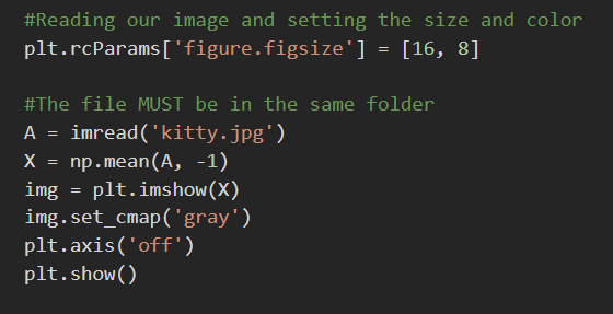
When we call the plt.show function, it will display our new photograph in a grayscale.

Now, let’s see where the magic begins. We’re going to compute the SVD Algorithm using the function imported in NumPy.

At first, this might be tricky to watch, but what we’re doing here is extracting the diagonal entries in the Sigma matrix and arranging them in descending order. Then, iteratively, we’re going to select the first k values of every matrix. Selecting the U’s columns and VT’s rows. This way we’re going to watch the closest way we can approach the original image.
When calling the last function, it will show us three different approaches with the given k values.
The first one won’t show us anything clear, but we can guess that the image is showing us a cat because of the pointy ears.

In the next picture, we can clearly see a cat, but obviously, it’s a blurry image, so we can’t appreciate the details the original image has.

The final image has a greater number of k values, which allows us to see a more clear picture. Sure, it has some details missing, but it’s a great number of values we can use for compression. This image’s great for future use in a project we want to work on, maybe a cat album page or a veterinary site.

In conclusion
The Singular Value Decomposition Algorithm is a powerful tool for dimensionality reduction, in this article, we were capable of making a quick review of some math terms that helps us know how this algorithm works and how can it be applied in important fields likewise image compression.
In the case of image compression, being of great help when it comes to transmission and storage reduction, we noticed that simple use of this algorithm is achieved by choosing an adequate value of k. While we’re increasing this number, the original matrix will be reconstructed almost like the original image. That way, we can notice that this is a simple algorithm since it doesn’t have a high computational complexity.
But image compression is not the only thing that this algorithm work with but with other elements like a database itself or video compressions. I’ll encourage you to make further reading and practice with the algorithm we worked on in the Python tutorial sections. Nice coding!
References:
Pillow, J. (2018). Statistical Modeling and Analysis of Neural Data, Spring 2018. Pillow Lab @ Princeton. Retrieved August 12, 2022, from http://pillowlab.princeton.edu/teaching/statneuro2018/
Serrano.Academy. (2020). Singular Value Decomposition (SVD) and Image Compression [Video]. YouTube. https://www.youtube.com/watch?v=DG7YTlGnCEo&t=33s&ab_channel=Serrano.Academy
Swathi, H. R., Sohini, S., Surbhi, & Gopichand, G. (2017). Image compression using singular value decomposition. IOP Conference Series: Materials Science and Engineering, 263, 042082. https://doi.org/10.1088/1757-899x/263/4/042082