
PCA Algorithm Tutorial in Python

Principal Component Analysis (PCA)
Principal Component Analysis is an essential dimensionality reduction algorithm. It entails lowering the dimensionality of data sets to reduce the number of variables. It keeps the most crucial information in this manner. This method is a helpful tool capable of several applications such as data compression or simplifying business decisions. Keep reading if you want to learn more about this algorithm.
The focus of this algorithm is to reduce the data set to make it simpler while retaining the most valuable possible information. Simplifying the dataset makes it easier to manipulate and visualize the data, resulting in quicker analysis.
Already understand how PCA works? Jump forward to the code!
How is PCA possible?
There are multiple ways to calculate PCA. We’re going to explain the widely used: Eigendecomposition of the covariance matrix.
An eigendecomposition is the factorization of a matrix in linear algebra. We can use a mathematical expression to represent this through the eigenvalues and eigenvectors. These concepts will be explained in section 3: “Calculate the Eigendecomposition of the Covariance Matrix”. Having this in mind, let’s dive further into the five steps to compute the PCA Algorithm:
1. Standardization
Standardization is a form of scaling in which the values are centered around the mean and have a unit standard deviation. Allowing us to work, for example, with unrelated metrics.
It means every feature is standardized to have a mean of 0 and a variation of 1, putting them on the same scale. In this manner, each feature may contribute equally to the analysis regardless of the variance of variables or if they are of different types. This step prevents variables with ranges of 0 to 100 from dominating the ones with values of 0 to 1, making a less biased and more accurate outcome.
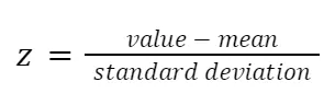
Standardization can be done mathematically by subtracting the mean and dividing by the standard deviation for each variable value. The letter z represents the standard score.
Once standardized, every feature will be on the same scale.
2. Covariance Matrix Computation
The covariance matrix is a square matrix that displays the relation between two random features, avoiding duplicated information since the variables we’re working with sometimes can be strongly related.
E.g. let’s imagine we have milk and coffee, they are different drinks that people usually drink. In conducting a survey, we can ask some people which beverage gives them more energy noting their score from 0 to 5. The results will be the data points we can collect to build our covariance matrix. The following table represents collected data from three subjects, having two variables “C” and “M”, that identify coffee and milk, respectively.

This table can be represented in a graph like the following.

As we can see, the horizontal axis represents Coffee, while the vertical axis represents Milk. Here, we can notice some vectors created with the values shown in the previous table, and every vector is labeled according to the subjects’ answers. This graph can be represented as a covariance matrix. A covariance matrix with these features will compare the values each feature has and will proceed with the calculations.
This covariance matrix is calculated by transposing the matrix A and multiplying by itself, then dividing by the number of samples. Represented as the formula below:

Resulting in matrices like these:

We have two instances of Covariance Matrices here. One is a 2x2 matrix, while the other is a 3x3 matrix. Each with the number of variables according to its dimension. These matrices are symmetric with respect to the main diagonal. Why?
The covariance of a variable with itself represents the main diagonal of each matrix.
cov(x,x)= var(x)
Also, we have to take into account that covariance is commutative.
cov(x,y)= cov(y,x)
That way, we see that the top and bottom triangular parts are therefore equal, making the covariance matrix symmetric with respect to the main diagonal.
At this point, we need to take into account the sign of the covariance. If it’s positive, both variables are correlated; if it’s negative, they’re inversely correlated.
3. Calculate the Eigendecomposition of the Covariance Matrix
In this phase, we will compute the eigenvectors and eigenvalues of the matrix from the previous step. That way, we’re going to obtain the Principal Component. Before entering into the process of how we do this, we’re going to talk about these linear algebra concepts.
In the realm of data science, eigenvectors and eigenvalues are both essential notions that scientists employ. These have a mathematical basis.
An eigenvector is a vector that represents an approximation to a large matrix. This vector won’t change by any transformation; instead, it becomes a scaled version of the original vector. The scaled version is caused by the eigenvalue, that’s simply a calculated value that stretches the vector. Both come in pairs, with the number of pairings equaling the number of matrix dimensions.
Principal Components, on the other hand, being the major focus of this approach, are variables formed as linear combinations of the starting features. The primary goal of the principal components is to save the most uncorrelated data in the first component and leave the remainder to the following component to have the most residual information and so on until all the data is saved.
This procedure will assist you in reducing dimensionality while retaining as much information as possible and discarding the components with low information.
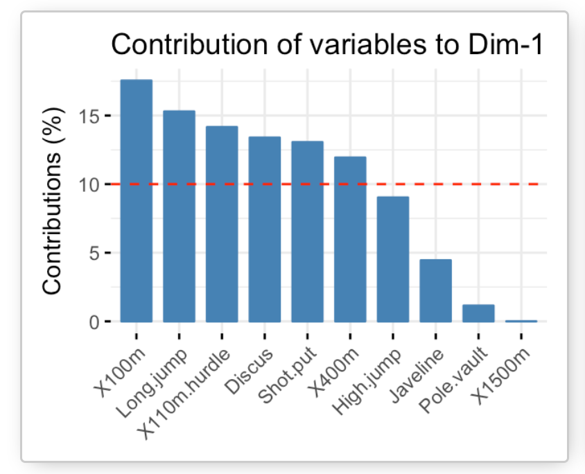
Example of a Principal Component, showing the contributions of variables in Python. Image Source: plot — Contributions of variables to PC in python — Stack Overflow
Now we have all the concepts clear. The real question is how can PCA Algorithm construct the Principal Component?
All of the magic in this computation is due to the eigenvectors and eigenvalues. Eigenvectors represent the axes’ directions where the maximum information is permitted. These are referred to as Principal Components. Eigenvalues, as we know, are values attached to the eigenvectors, giving the amount of variance that every principal component has.
If you rank the eigenvectors in order of every eigenvalue, highest to lowest, you’re going to get the principal components in order of significance, just like the following picture.

Eigenvectors and eigenvalues of a 2-dimensional covariance matrix. Image source: A Step-by-Step Explanation of Principal Component Analysis (PCA) | Built In
With the principal components established, the only thing left to do is calculate the proportion of variation accounted for by each component. It is possible to do this by dividing the eigenvalues of each component by the sum of eigenvalues.
4. Feature Vector
A Feature Vector is a vector containing multiple variables. In this case, it is formed with the most significant Principal Components, which means, the one with the vectors corresponding to the highest eigenvalues. The number of the principal component we want to add to our feature vector is up to us and up to the problem we’re going to solve.
Following the same example of the last step, knowing that 1>2, our feature vector can be written this way:

Feature Vector with two Principal Components. Image source: A Step-by-Step Explanation of Principal Component Analysis (PCA) | Built In
Also, we know that our second vector contains less relevant information, which is why we can skip it and only create our feature vector with the first principal component.

Feature Vector with only a Principal Component. Image Source: A Step-by-Step Explanation of Principal Component Analysis (PCA) | Built In
We need to take into consideration that reducing our dimensionality will cause information loss, affecting the outcome of the problem. We can discard principal components when it looks convenient, which means when the information of those principal components we want to discard is less significant.
5. Recast the Data Along the Axes of the Principal Components
Because the input data is still in terms of the starting variables, we must utilize the Feature Vector to reorient the axes to those represented by our matrix’s Principal Components.
It can be done by multiplying the transposed standardized original data set by the transpose of the Feature Vector.

Now that we finally have the Final Data Set, that’s it! We’ve completed a PCA Algorithm.
PCA Python Tutorial
However, when you have basic data, such as the previous example, it is quite straightforward to do it with code. When working with massive amounts of data, scientists are continually looking for ways to compute this Algorithm. That’s why we’re going to complete an example in Python, you can follow along in this Jupyter Notebook.
The first thing we’re going to do is import all the datasets and functions we’re going to use. For a high-level explanation of the scientific packages: NumPy is a library that allows us to use mathematical functions, this will help us to operate with the matrices (also available thanks to this library).
Seaborn and Matplotlib are both used to generate plots and graphics. Matplotlib is also used as an extension of NumPy, including more mathematical functions.
Sklearn is the reserved word for scikit-learn, a machine learning library for Python, it has some loaded datasets and various Machine Learning algorithms.

Importing Data and Functions
Next, we will declare a class called PCA, which will have all the steps we learned previously in this blog.

PCA Class and Functions
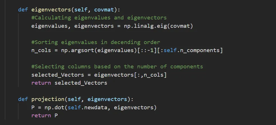
Functions for Eigenvectors and Projection
These functions are pretty intuitive and easy to follow. The next step is to implement this PCA Class. We’re going to initialize the variables we’re going to use.

Initialization of Variables
Here we can notice we’re using the datasets library, extracted from scikit-learn. Then, we assigned those values to our variables. Scikit-learn comes with various datasets, we’re going to use the known ‘Toys datasets’. These are small standard datasets, used mostly in algorithms examples or tutorials.
Specifically, we’re loading the diabetes dataset. According to the authors, this data is based on “Ten baseline variables, age, sex, body mass index, average blood pressure, and six blood serum measurements were obtained for each of n = 442 diabetes patients, as well as the response of interest, a quantitative measure of disease progression one year after baseline.”
Following the code, now we’re going to initialize the class and start calling out the functions of the class. When running the code, we can have the following outcome.

PCA Initialization

PCA Example in Python
To watch the differences between the original datasets, we can just call the first two functions of the class, throwing the next scatterplot:

Scatterplot Graph of Diabetes Dataset
If we do the whole PCA process, we can better visualize the data in this way:

PCA Graph of Diabetes Dataset
Now, we’ve learned about the key computing procedures, which included some crucial linear algebra basis.
In Conclusion
The Principal Component Analysis is a straightforward yet powerful algorithm for reducing, compressing, and untangling high-dimensional data. It allows us to isolate the data more clearly, and use it for various machine learning methods.
Since the original data was reduced in dimensionality terms, retaining trends and patterns, we can notice that the final output of this algorithm is easier to manipulate, making further analysis much easier and faster for the machine learning algorithm, allowing us to forget unnecessary variables and some problems like the curse of dimensionality.
The next step is to use your new transformed variables with other machine learning algorithms to better understand your data and finally finish your research. If you want a general guide on the existing different machine learning methods and when to use them, you can check my previous entry on “Machine Learning Algorithms”.
Follow me here for more AI, Machine Learning, and Data Science tutorials to come!

You can stay up to date with Accel.AI; workshops, research, and social impact initiatives through our website, mailing list, meetup group, Twitter, and Facebook.
References:
A guide to principal component analysis (PCA) for Machine Learning. A Guide to Principal Component Analysis (PCA) for Machine Learning (2020). Available at: https://www.keboola.com/blog/pca-machine-learning. (Accessed: 14th February 2022).
Scikit-learn: Machine Learning in Python, Pedregosa et al., JMLR 12, pp. 2825–2830, 2011.
Jaadi, Z. A step-by-step explanation of principal component analysis (PCA). Built In (2021). Available at: https://builtin.com/data-science/step-step-explanation-principal-component-analysis. (Accessed: 14th February 2022).
Tsesmelis, T. Introduction to principal component analysis (PCA). OpenCV Available at: https://docs.opencv.org/4.x/d1/dee/tutorial_introduction_to_pca.html. (Accessed: 16th February 2022).
Lanhenke, M. Implementing PCA from scratch. Medium (2021). Available at: https://towardsdatascience.com/implementing-pca-from-scratch-fb434f1acbaa. (Accessed: 15th February 2022).