
K-Means Tutorial in Python
Hi everyone,
Welcome back to my series of Machine Learning Algorithms Tutorials, this time we’ll be checking on K-Means, one of the most popular and powerful clustering algorithms in Machine Learning. In this article, I will explain what it is, how it works, and why it’s useful for finding patterns in data. We’ll obviously have our tutorial in Python as well!
I hope you enjoy reading this article as much as I enjoyed researching and writing it. With this series, I developed a fascination for Machine Learning and how it can help us solve complex problems and make better decisions. If you share this passion, then you are in the right place. Let’s dive in!
K-Means is one of the popular and simple clustering algorithms. It is an unsupervised learning technique that aims to partition a set of data points into a number of groups (called clusters) based on their similarity.
The basic idea of K-Means is to assign each data point to the cluster whose center (called centroid) is closest to it. The centroid of a cluster is the average of all the data points in that cluster. The algorithm iterates until the centroids stop changing or a maximum number of iterations is reached.
We need to know what the algorithm needs to work, in this case, K-means requires the following inputs:
The number of clusters (k), where we specify the number of clusters we want the algorithm to group the data into.
Data, that need to be clustered. Each data point should have a set of features or attributes that describe it.
Initial centroids for each cluster. These centroids can be randomly selected from the data points or manually specified.
Determining the optimal number of clusters (k) is an important step in using the k-means algorithm effectively. There are several methods that can be used to estimate the optimal value of k, including:
Elbow method, which involves plotting the sum of squared distances between each data point and its assigned centroid for different values of k. The value of k at which the rate of decrease in the sum of squared distances slows down and forms an elbow-like shape is considered the optimal number of clusters.
Silhouette method involves calculating the silhouette score for different values of k. The silhouette score measures how similar a data point is to its assigned cluster compared to other clusters. The value of k that maximizes the average silhouette score is considered the optimal number of clusters.
Gap statistic method, this technique involves comparing the within-cluster variation for different values of k to a null reference distribution. The value of k that maximizes the gap statistic is considered the optimal number of clusters.
It’s important to note that these methods are not foolproof and may not always give a clear indication of the optimal number of clusters. Therefore, it’s often useful to try multiple methods and compare the results to choose the best value of k.
The next thing to do is to initialize the centroids, there are different ways to initialize the k centroids in this algorithm, including:
Random initialization: k centroids are randomly selected from the data points. This is a simple and commonly used method, but it may result in suboptimal clustering if the initial centroids are not representative of the data distribution.
K-means++ Initialization: aims to select k centroids that are far apart from each other and representative of the data distribution. It involves selecting the first centroid randomly from the data points and then selecting subsequent centroids based on the distance from the previously selected centroids. This method typically results in better clustering performance than random initialization.
Manual Initialization: in some cases, the user may have prior knowledge about the data and the expected clusters, and can manually specify the initial centroids.
Notice that the choice of initialization method can affect the clustering result, so it’s often recommended to run the algorithm multiple times with different initializations and choose the best result.
Once we have our initialization method defined, we can start with our iterative process which consists of calculating the distance between the points and each centroid, assigning the points to each cluster, and updating the centroid positions.
For each data point in the dataset, the algorithm calculates the Euclidean distance between the point and each centroid. The Euclidean distance is simply the straight-line distance between two points in a Euclidean space, such as a two-dimensional plane. This metric is more used because of its simplicity to compute, and it's also an intuitive distance metric that can be easily understood and visualized.
Moreover, the Euclidean distance is suitable for continuous data and mathematical models. However, there are cases where the Euclidean distance may not be appropriate, such as text clustering problems. In this situation is commonly used the cosine distance metric, this one measures the angle between two vectors.
The choice of distance metric depends on the nature of the data and the problem at hand. It is always a good practice to explore different metrics.
Once the distance is calculated, the algorithm assigns each data point to the cluster with the closest centroid.
After this step, the algorithm recalculates the centroid positions, which represents the mean of all data points assigned to each cluster. Next thing to do is repeat this iterative process until convergence is reached. It is achieved when the assignment of data points to clusters no longer changes or when the change is below a predefined threshold.
The final output of the algorithm is a set of k clusters, each represented by its centroid, and a label for each data point indicating its assigned cluster. Finally, describe how to evaluate the quality of the clustering result using metrics such as the within-cluster sum of squares of silhouette score.
After providing an overview of the k-means algorithm, it’s important to discuss its strengths and limitations, understanding these is important for making informed decisions about its use in different applications.
Among its benefits we can include the following:
It’s computationally efficient and suitable for large datasets, this is because the algorithm only requires a few simple computations for each iteration, making it a suitable choice for clustering tasks where efficiency is an important consideration.
It is easy to understand and implement, due to not requiring advanced mathematical or statistical knowledge. Making it accessible to practitioners with varying levels of expertise in data science and machine learning.
It can handle data with a large number of dimensions. K-means is able to find patterns and structure in high-dimensional data, making it a valuable tool in many applications.
However, K-Means is not without its limitations, including:
The algorithm relies on the initial selection of centroids, which can affect the final clustering results. As we previously discussed, it is recommended to run the algorithm multiple times with different initializations so it can help to mitigate, not eliminate, this limitation.
K-means assumes that the clusters are spherical, which can lead to incorrect cluster assignments when clusters are non-spherical. In real-world datasets, clusters can have complex shapes and structures that do not fit the spherical assumption of k-means. In these cases, more advanced clustering algorithms such as density-based clustering or hierarchical clustering may be more appropriate.
The algorithm struggles with identifying clusters of varying sizes and densities. This is because the algorithm assigns data points to the closest centroid, which can result in one large cluster and several small clusters.
Overall, understanding the limitations of k-means is important for making informed decisions about when and how to apply the algorithm. It is good to notice that despite these limitations, K-Means remains one of the most widely used clustering algorithms because of its simplicity and efficiency and has not deterred its use in various domains.
The K-Means algorithm has several applications in various disciplines, including:
Market segmentation: K-means clustering is often used in marketing to segment customers based on their behavior, preferences, and demographics. By grouping customers with similar characteristics, companies can tailor their marketing strategies to each segment and improve customer satisfaction and loyalty.
Image segmentation: segmentation of images based on their color or texture features. This technique is commonly used in image compression, object recognition, and image retrieval.
Anomaly detection: it can be used for anomaly detection in various fields, such as finance, cybersecurity, and fraud detection. By clustering normal data points and identifying outliers that do not belong to any cluster, k-means can help detect unusual patterns that may indicate fraudulent or suspicious activity.
Bioinformatics: clustering of genes, proteins, or samples based on their expression levels or sequence similarity. This technique can help identify patterns in large biological datasets and enable researchers to study the relationships between different biological entities.
Social Network Analysis: K-means clustering can be used in social network analysis to cluster users based on their behavior, interests, or social connections. By identifying groups of users with similar characteristics, researchers can gain insights into the structure and dynamics of social networks and predict user behavior.
While K-Means is a very effective algorithm with plenty of applications, it may not be suitable for some situations like categorical data, as previously said. In the same way, there could be some flaws that led to the development of variants and extensions of this algorithm, including K-Modes.
K-Modes is a clustering algorithm that is specifically designed for categorical data and is based on the same principles as K-Means. In this way, the algorithm represents an important extension and highlights the ongoing development of clustering techniques to meet the diverse needs of researchers and practitioners.
There are several variants and extensions of the K-Means algorithm that have been proposed. Some examples are K-Medoids, Fuzzy C-Means, and K-Prototype. The first one replaces the mean calculation with the selection of a representative data point from each cluster, known as a medoid, making it more robust to outliers and noise in the data.
Fuzzy C-Means assigns a degree of membership to each data point for every cluster. This allows for more nuanced clustering and can be useful when there is uncertainty or overlap between clusters. For example, in image segmentation, a pixel may belong to multiple regions with different colors, and this type of clustering can provide a more accurate representation of the underlying structure of the data.
Finally, the K-Prototype extension is a hybrid algorithm that combines both K-Means and K-Modes to cluster datasets with both numeric and categorical data. It assigns a weight to each feature based on its type and uses this to calculate the distance between data points.
These variants and extensions demonstrate the ongoing efforts to improve and adapt clustering algorithms to better suit the needs of different applications and types of data.
Python Tutorial
To ensure compatibility, it is recommended to use an Anaconda distribution for this tutorial. However, if you don’t have Anaconda installed and you want to use your trusted Kernel, you can manually install the required packages using pip. You can execute the provided code block by uncommenting from the “import sys” line onwards to automatically install the necessary packages.

To perform this tutorial, we need to import several essential libraries in Python.

We import NumPy, a powerful library for numerical operations on arrays, which provides efficient mathematical functions and tools. Next, we import pandas, a widely used data manipulation and analysis library that allows us to work with structured data in a tabular format.
To visualize the results of our clustering analysis, we import matplotlib.pyplot, a plotting library that enables us to create types of charts and graphs. This will help us understand the patterns and relationships within the data.
For the actual clustering process, we import scikit-learn’s KMeans module. To ensure accurate results, we also import the StandardScaler module from scikit-learn’s preprocessing submodule. It is used for feature scaling, which helps to normalize the data and improve the performance of the clustering algorithm.
Lastly, we import silhoutte_score from scikit-learn’s metric module. The Silhouette Score is a metric used to evaluate the quality of the clustering results. It measures how well each data point fits within its assigned cluster.

Next, we’re using the housing data from a CSV file called “housing.csv”, you can reach this file in the following Kaggle page: California Housing Prices | Kaggle. We specify the columns of interest (longitude, latitude and median_house_value).
Then we remove any rows that have missing values (NaN). This ensures that we are working with a clean and complete dataset for further analysis.
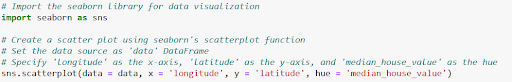
Now we import the seaborn library to create a scatter plot. We indicate to the function the axis values and the hue, which will help us understand the relationship between the longitude and latitude coordinates of the housing data with the median house value. It displays the following scatter plot.

We create an instance of the StandardScaler class from scikit-learn’s preprocessing module. This will help us to normalize the data and bring it to a standard scale.

When we perform the fit.transform, the method calculates the mean and standard deviation of each feature in the dataset and applies the scaling transformation accordingly. We save this value in the data_scaled variable.
By scaling the features, we ensure that they have a similar range and variance, which can be beneficial for certain machine learning learning algorithms and data analysis techniques.
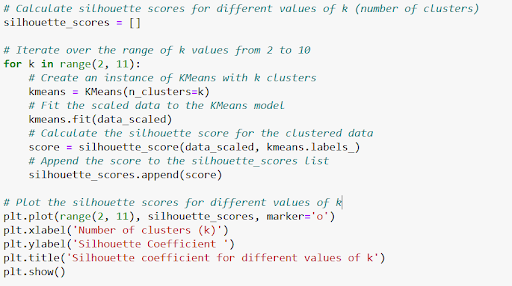
In this step, the initialize an empty list called “silhouette_scores” to store the scores. Then, we iterate through the range of k values from 2 to 10. For each value of k, we create an instance of the KMeans class with k clusters and fit the scaled data to the model.
Next, we calculate the silhouette score for the clustered data using the silhouette_score function, which measures the quality of the clustering results. The resulting score is appended to the silhouette_score list.
Finally, we plot the silhouette scores against the values of k, where the x-axis represents the number of clusters (k), and the y-axis represents the silhouette coefficient. The plot is labeled with appropriate axes labels and a title, and displayed.

After plotting this graph of the silhouette coefficient for different values of k, we can analyze the results to determine the optimal number of clusters for our data. We need to identify the value of k that corresponds to the peak or highest silhouette coefficient on the graph. This will be the number of clusters that yield the most distinct and well-separated groups within the data. In this case, k equals the number 2.

We set the number of clusters (k) to 2, partitioning the data into two distincts groups. We then create an instance of the KMeans class with the specified number of clusters. We use K-Means++ as our init method, which is widely used and helps improve the convergence of the algorithm. Additionally, we set a random state of 42 to ensure reproducibility of the results.
After that, we fit the scaled data to the KMeans model using the fit() method. This process calculates the cluster centroids and assigns each data point to its corresponding cluster based on the proximity of the centroids.

Finally we obtain the clusters and centroid labels and set the scatter plot labels to show our graph.

The cluster centroids are marked as red X’s. For furthermore exploration of this algorithm, you can visit our GitHub Repository where you can access the complete code for convenient execution and customization.
In conclusion
K-Means is a popular clustering algorithm in machine learning that aims to partition data points into clusters based on their similarity. It is an unsupervised learning technique that can find patterns in data.
The algorithm works by iteratively assigning data points to the cluster with the closest centroid and updating the centroids based on the assigned points. It continues this process until convergence.
K-Means requires specifying the number of clusters (k), providing the data to be clustered, and initializing the centroid. Determining the optimal value of k can be done using methods like the elbow method, silhouette method, or gap statistic method.
This technique has strengths such as computational efficiency, ease of implementation, and the ability to handle high-dimensional data. However, it has limitations such as sensitivity to initial centroid selection and the assumption of spherical clusters.
Evaluation of the clustering result can be done using metrics like the within-cluster sum of squares or silhouette score. K-Means finds applications in market segmentation, image segmentation, anomaly detection, bioinformatics, and social network analysis.
Are you eager to delve deeper into the fascinating world of machine learning and explore more powerful algorithms like K-Means? If so, I invite you to continue your learning journey and unlock the potential of this exciting field. You can explore our other tutorials and resources to provide in-depth explanations and practical examples that can guide you step-by-step through implementing Machine Learning algorithms.
Additionally, consider joining our community, where you can engage with like-minded individuals, exchange insights, and collaborate on different kinds of projects. The collective wisdom and support can enhance your learning experience and open doors to exciting opportunities. The possibilities are waiting for you, start your journey now!
References
Babitz, K. (2023). Introduction to k-Means Clustering with scikit-learn in Python. https://www.datacamp.com/tutorial/k-means-clustering-python
K-Means Clustering Algorithm - JavatPoint. (n.d.). www.javatpoint.com. https://www.javatpoint.com/k-means-clustering-algorithm-in-machine-learning
Li, Y., & Wu, H. (2012). A clustering method based on K-Means algorithm. Physics Procedia, 25, 1104–1109. https://doi.org/10.1016/j.phpro.2012.03.206
Mannor, S., Jin, X., Han, J., Jin, X., Han, J., Jin, X., Han, J., & Zhang, X. (2011). K-Means clustering. In Springer eBooks (pp. 563–564). https://doi.org/10.1007/978-0-387-30164-8_425
T. Kanungo, D. M. Mount, N. S. Netanyahu, C. D. Piatko, R. Silverman and A. Y. Wu, "An efficient k-means clustering algorithm: analysis and implementation," in IEEE Transactions on Pattern Analysis and Machine Intelligence, vol. 24, no. 7, pp. 881-892, July 2002, doi: 10.1109/TPAMI.2002.1017616.