
DBSCAN Algorithm Tutorial in Python
Density-based Spatial Clustering of Applications with Noise (DBSCAN)
In my previous article, HCA Algorithm Tutorial, we did an overview of clustering with a deep focus on the Hierarchical Clustering method, which works best when looking for a hierarchical solution. In the case where we don’t want a hierarchical solution and we don’t want to specify the number of clusters we’re going to use, the Density-based Spatial Clustering of Applications with Noise, abbreviated DBSCAN, is a fantastic choice.
This technique performs better with arbitrary-shaped clusters - clusters without a simple geometric shape like a circle or square- with noise, which means those clusters have data points that don’t belong to them. DBSCAN also aids in outlier detection by grouping points near each other with the use of two parameters termed Eps and minPoints.
Eps, also known as Epsilons, are the radius of the circles we will generate around every data point, while minPoints are the smallest number of data points that must surround a single central data point in order to make it a core point.

Image Extracted from DBSCAN Clustering Algorithm in Machine Learning - KDnuggets
All points that are not within another point’s Eps distance and do not have the corresponding number of minPoints within their own Eps distance are called noise or outliers.
The selection of Eps and minPoints must be done with specific focus because a single change in values might influence the entire clustering process. But how can we know the recommended values for our problems?
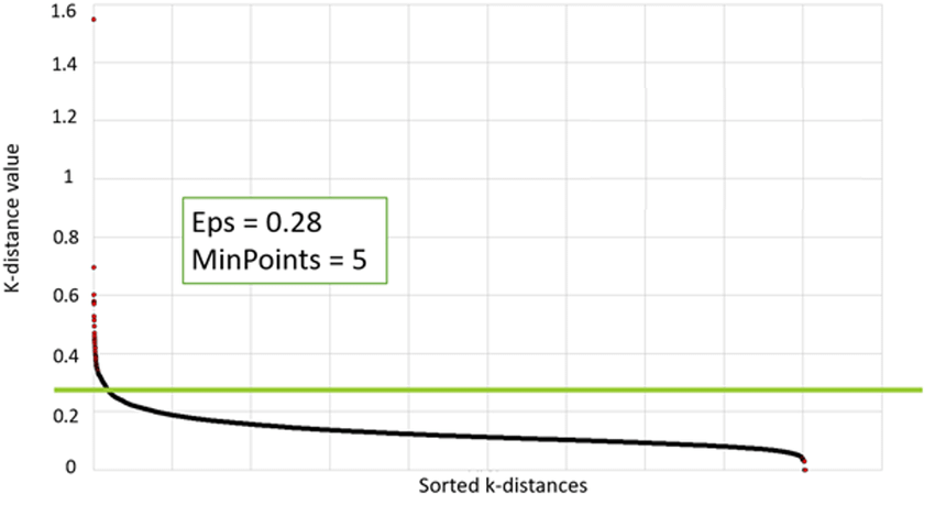
K-distance plot for the DBSCAN tuning parameters. Image extracted from (PDF) A Data-Driven Energy Platform: From Energy Performance Certificates to Human-Readable Knowledge through Dynamic High-Resolution Geospatial Maps
We can use some estimations according to our problem’s dataset. We should pick Eps depending on the dataset's distance and we may utilize a k-distance graph to assist us. We should be aware that a small number is always preferable since a large value would combine more data points per cluster, and some information can be lost.
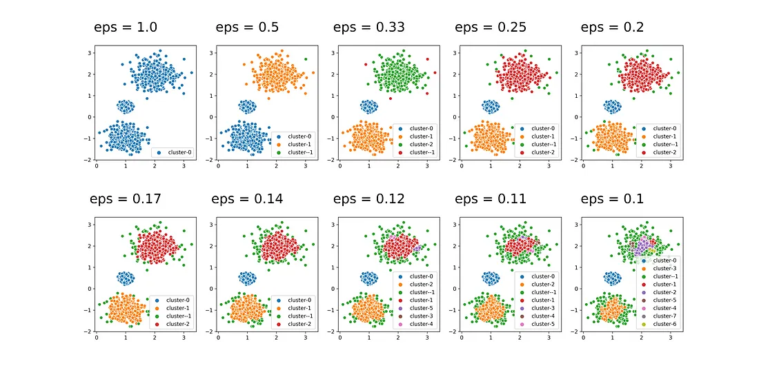
Example of variation of eps values. Image extracted from How to Use DBSCAN Effectively
It is evident that the most optimal results are achieved when the value of “eps” lies between 0.17 and 0.25. When the value of eps is smaller than this range, there is an excessive amount of noise or outliers, represented by the green color in the plot. On the other hand, when it’s bigger, the clusters become too inclusive like the eps value of 1, when it’s a single cluster.
The value of minPoints is according to the number of data points we have. However, we must consider that the minimum value can be our dataset dimension, it means the number of features we’re working with plus 1, while we don’t have a maximum value number. Therefore, the larger the data collection, the greater the minPoints value we should select.
Now that we understand the concepts, let’s see how this algorithm works. The first step is to classify the data points. The algorithm will visit all data points but arbitrarily select one to start with. If the iteration confirms that there are the corresponding number of minPoints in the radius Eps around the datapoint selected, it considers these points part of the same cluster.
Then the algorithm will repeat the process with the neighbors just selected, possibly expanding the cluster until there are no more near data points. At that point, it will select another point arbitrarily and start doing the same process.
It can be possible to have points that don’t get assigned to any clusters, these points are considered noise or outliers, and these will be discarded from our algorithm once we stop iterating through the dataset.
Now that we have knowledge of how this algorithm works, let’s compute it with a simple Tutorial in Python.
Python Tutorial
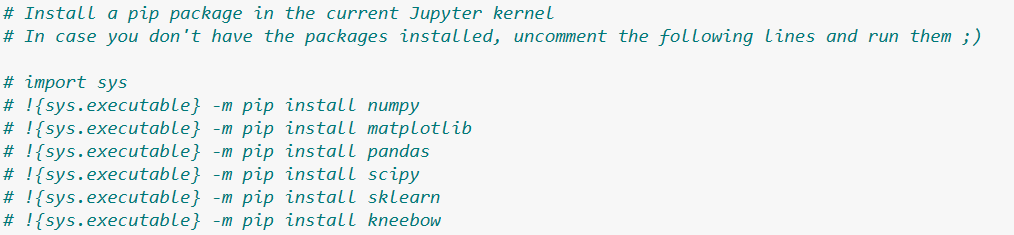
As always, let’s use an Anaconda distribution, but in case you are not related to it, you can previously install the packages by executing some pip installing or you can run the following code block, beginning the uncommenting from the “import sys”:
Now, we’re going to make some basic imports to use them in our program.

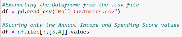
For this tutorial, we’ll use a dataset known from our previous article, a list of mall customers (extracted from Machine Learning A-Z: Download Codes and Datasets - Page - SuperDataScience | Machine Learning | AI | Data Science Career | Analytics | Success). And we’re going to use, as before, the annual income and spending score values.
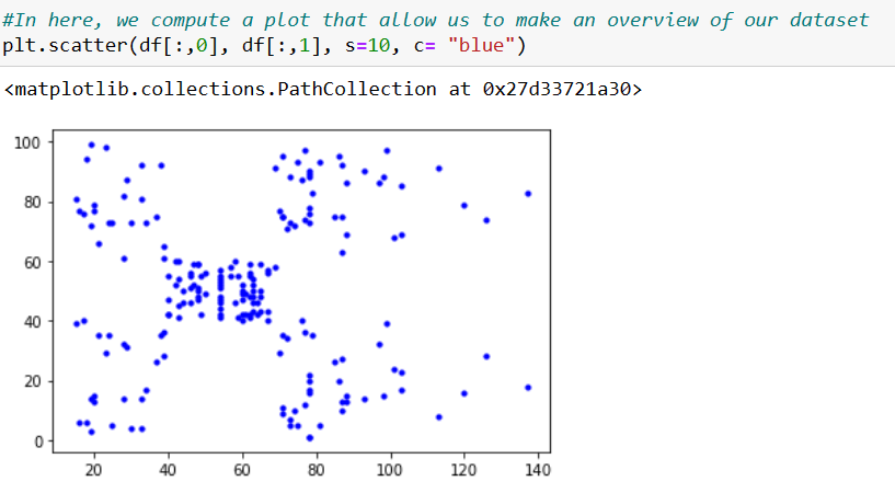
At this point we have our data points on memory, let’s compute a plot where we can see those points for a clear view of this example.
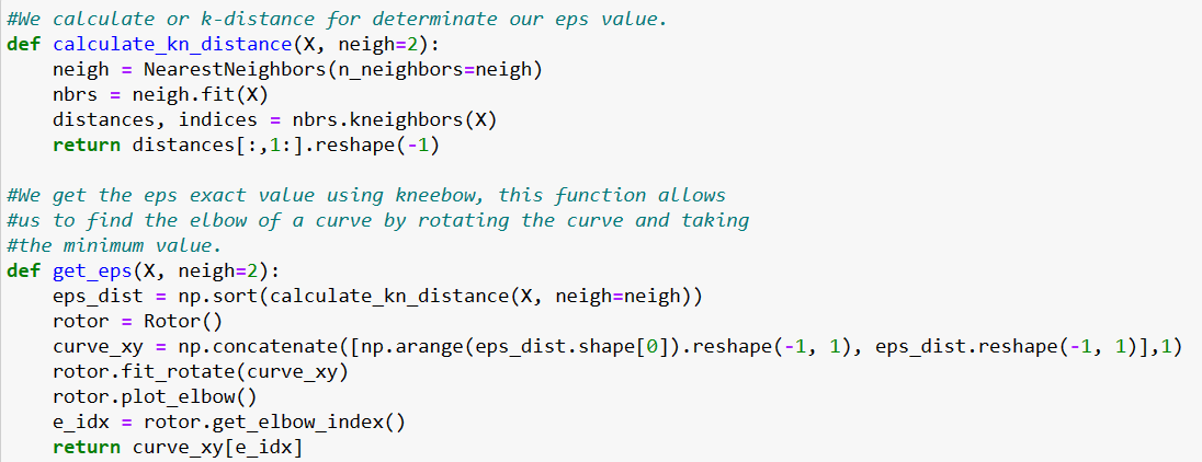
As previously mentioned, to compute this algorithm we need some defined parameters: Eps and minPoints. Although there’s not an automatic way to determine minPoints value, we can compute some functions that will allow us to have our Eps. This will be made by computing the k-distance between all points in the dataset, the elbow of the curve will give us an approximation of the Eps value.
In this case when we call a function, we will get a float number, or a decimal value. We will have to round it.
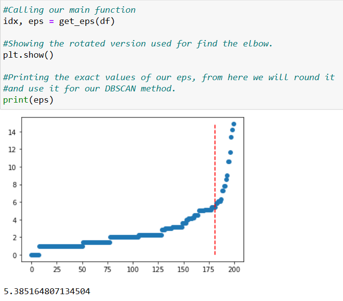
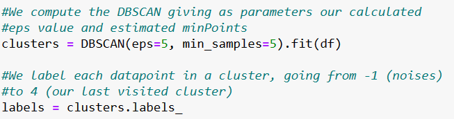
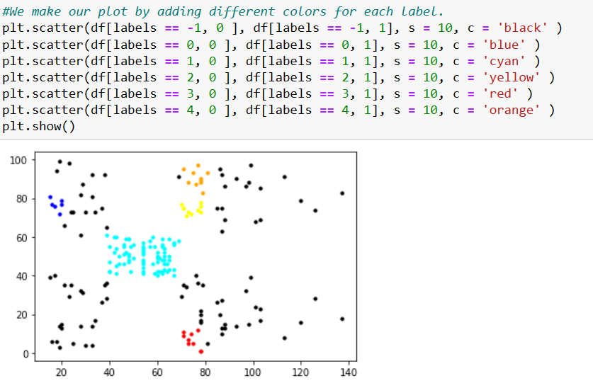
In this case, we will have an Eps value of 5, which will be our entry to our next function allowing the estimated minPoints. Next, we will give a label to every cluster, going from -1 (representing the noises or outliers) to 4 (our last visited cluster).
Finally we will make our scatterplot, assigning colors for each of the labels. Finishing this tutorial.
In conclusion, the DBSCAN algorithm is a powerful and versatile method for clustering data in a variety of applications. It is particularly well-suited for handling data with irregular shapes and varying densities, and is able to identify noise points and outliers in the data. DBSCAN is also relatively easy to implement and does not require prior knowledge of the number of clusters in the data, making it a popular choice for exploratory data analysis.
However, like any clustering algorithm, DBSCAN has some limitations and assumptions that should be considered when applying it to real-world data. For example, it assumes that clusters are dense regions separated by areas of lower density, and may not perform well on data with very different density levels or noise points that are distributed throughout the data. Additionally, it requires careful selection of its parameters such as the neighborhood size and the minimum number of points required to form a cluster, which can affect the clustering results.
Overall, the DBSCAN algorithm is a valuable tool for data clustering and has been applied successfully in a wide range of fields including image processing, text mining, and bioinformatics. By understanding its strengths and limitations, researchers and practitioners can make informed choices about when and how to apply DBSCAN to their own data.
If you’re interested in exploring the code behind the project discussed in this article, I invite you to visit the corresponding repository on GitHub. There, you can find the source code and view it in action. By exploring the repository, you’ll gain a deeper understanding of how the project was built and how you might be able to use it for your own purposes. I’m available to answer any questions you may have, so don’t hesitate to reach out if you need support. You can find the link to the repository in the article’s footer or by visiting my GitHub profile. Happy coding!