
Hierarchical Clustering Algorithm Tutorial in Python
When researching a topic or starting to learn about a new subject a powerful strategy is to check for influential groups and make sure that sources of information agree with each other. In checking for data agreement, it may be possible to employ a clustering method, which is used to group unlabeled comparable data points based on their features. For example, you can use clustering to group documents by topics.
On the other hand, clustering can also be used in market segmentation, social network analysis, medical imaging, and anomaly detection.
There are different types of clustering algorithms, and their application goes according to the type of problem or approach we want to implement. For example, if you’re searching for a hierarchical method, which implies you’re attempting a multi-lever learning technique and learning at multiple grain-size spaces, you may use hierarchical clustering.
Hierarchical clustering is a prominent Machine Learning approach for organizing and classifying data to detect patterns and group items to differentiate one from another.

The hierarchy should display the data in a manner comparable to a tree data structure known as a Dendrogram, and there are two methods for grouping the data: agglomerative and divisive.
Before entering into the deep knowledge of this, we’re going to explain the importance of a dendrogram on clustering. Not only does it give a better representation of the data grouping, but it also gives us information about the perfect number of clusters we might compute for our number of data points.
The agglomerative method is the most common type of hierarchical clustering, consisting of a “bottom-up” approach in which each object starts in its cluster, called a leaf, and the two most comparable clusters are joined into a new larger cluster at each phase of the algorithm, called nodes.
It is an iterative method, repeated until all points belong to a single large cluster called root that will contain all the data.
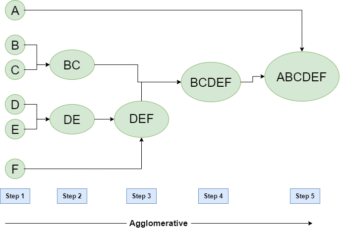
Image extracted from Hierarchical Clustering in Data Mining — GeeksforGeeks
The divisive method, which is the opposite of the agglomerative method, is not often used. This divisive approach is less typically employed in hierarchical clustering since it is more computationally costly, resulting in slower performance.
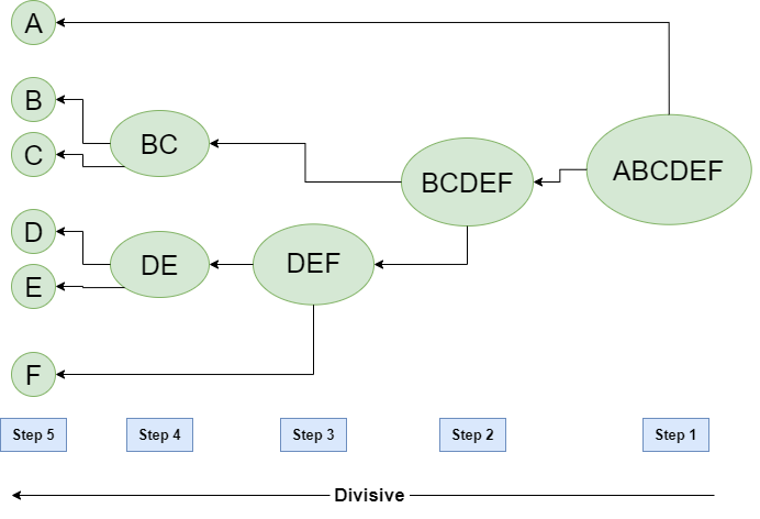
Image extracted from Hierarchical Clustering in Data Mining — GeeksforGeeks
To make this algorithm possible, using an agglomerative approach, we must complete the following steps:
The first step is to create a proximity matrix, computing the distance between each pair of data points, which means the distance between a data point and the others. It’s commonly used the euclidean distance function, given by the formula

Where

Having this in mind, the two data points we’re going to select will be according to our chosen linkage criteria. These criteria should be chosen based on theoretical concerns from the domain of application. There are a commonly used few of them:
Min Linkage, also known as single-linkage, is the calculation of distance between the two most comparable components of a cluster, which means the closest data points. It can also be defined as the minimum distance between points. The Min technique has the benefit of being able to handle non-elliptical forms properly. One of its drawbacks is that it is susceptible to noise and outliers.
Max Linkage, also known as complete linkage, is based on the two least similar bits of a cluster, or the same thing as the maximum distance between points. This linkage method is more vulnerable to noise and outliers than the MIN technique. It also can separate massive clusters and prefers globular clusters.
Centroid Linkage, which calculates the distance between the centroids of each cluster.
Average Linkage, defines cluster distance as the average pairwise distance between all pairs of points in the clusters.
When there are no theoretical concerns in our problem, it’s very helpful to use linkage criteria called Ward Linkage. This method examines cluster variation rather than calculating distances directly, reducing variance between clusters. This is accomplished by lowering or reducing the sum of squared distances between each cluster’s centroids. This method comes with the great power of being more resistant to noise and outliers. Now that you’ve calculated the distance using the according linkage criteria, you can merge the data points, creating a new cluster for each pair. After that, all you have to do is keep iterating until you have a single cluster. You may accomplish this by generating a new proximity matrix and computing the distances using the same linking criteria as before.
Tutorial in Python
Now that we’ve passed through all the basic knowledge, we’re ready to enter the python tutorial.
Remember that we’re using the Anaconda distribution, so in case you’re not using it, you’ll need to make the corresponding pip installs if you haven’t used these libraries before.
python -m pip install pip
pip install numpy
pip install pandas
pip install matplotlib
pip install scipy
pip install scikit-learn
Or you can uncomment the first code block in our Jupyter Notebook and execute it.

Now that you have installed the packages, we’re going to start coding. First, we need to import some basic libraries

For this example, we’re using a Comma-separated values file, here we’re using a list of mall customers (extracted from Machine Learning A-Z: Download Codes and Datasets — Page — SuperDataScience | Machine Learning | AI | Data Science Career | Analytics | Success). In this file, we obtain a list of customers and information about their annual income and their spending score, and our goal is to separate them into clusters using the HCA Algorithm.

Now we’re going to assign to a variable our wanted data points, which are the annual income and spending score by customer. It’s stored as an array with only the values.

The next step is to make some other imports.

Next, we generate a dendrogram using the scipy library importing, since our problem isn’t involved in a theoretical approach and we want a simple result, we’re using a ward linkage to treat it.


Taking a break from coding, we want to explain a little about the use of the Dendrogram. As you read before, the Dendrogram will give us the recommended number of clusters we will want to compute for our problem. But how can we know this? It’s as easy as drawing a parallel line so that it intercepts the greatest number of in this case vertical lines, making sure to not hit a horizontal line or ‘branching point.’

When two clusters are merged, the dendrogram will join them in a node, each node has a vertical distance which can be interpreted as the length on the y-axis. In our problem dendrogram.
We see that the intersection of the line with the most considerable distance, which means the greatest distance of a node, marks 5 different groups, which means it recommends five clusters for the problem. Having this in mind, we can advance to the next step.

Note: if the parameter “affinity” gives you an error, try changing it to “metric”, due to sklearn library’s deprecated versions.
We’re going to compute the Agglomerative Clustering; we’re going to use the Euclidean distance method and the same linkage criteria. Notice that we’re passing that we want 5 clusters for this problem.
Then, we just assign the data points to a corresponding cluster.
Finally, we’re going to compute our scatterplot and give each cluster a respective tag, according to their spending score and their annual income.
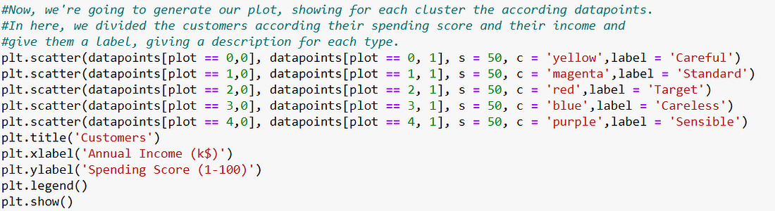
Throwing the final result, a scatter plot showing the five different clusters we computed and their respective legend.

In Conclusion
Hierarchical clustering is a robust method that works with unlabeled data, which is useful because most data, especially new or original data, does not come pre-labeled and thus requires a significant amount of time to classify/annotate. In this article, you learned the fundamental ideas of clustering, how the algorithm works, and some additional resources for a better understanding, such as dendrograms, euclidean distance computation, and linking criteria.
Despite its benefits, such as not utilizing a fixed number of clusters, we must note that hierarchical clustering does not perform well with huge data sets owing to the high space and complexity of the algorithm. This drawback is due to the need to calculate the pairwise distance between the datasets as discussed in our section on linkages, as well as the analysis of the dendrogram being too computationally intensive on huge data sets. Keeping these facts in mind we understand that on huge data sets Hierarchical clustering may take too long or require too much in the way of computational resources to provide useful results, but this type of algorithm is great for small to standard data sets and particularly useful in early understanding of unlabeled data.
You can stay up to date with Accel.AI; workshops, research, and social impact initiatives through our website, mailing list, meetup group, Twitter, and Facebook.

Join us in driving #AI for #SocialImpact initiatives around the world!
If you enjoyed reading this, you could contribute good vibes (and help more people discover this post and our community) by hitting the 👏 below — it means a lot!